Lab2-向量化计算

实验简介

1
2
3
4
5
6
7
8
9
10
11
12
Numpy 代码一般采用向量化(矢量化)描述,这使得代码中没有任何显式的循环,索引等,这样的代码有以下好处:

· 向量化代码更简洁,更易于阅读
· 更少的代码行通常意味着更少的错误
· 代码更接近于标准的数学符号

另外,向量化的代码能够规避掉 Python 中缓慢的迭代循环,被底层的实现更好的调度,如接入 BLAS 矩阵运算库,
从而实现更高的性能。

双线性插值是计算机视觉图像处理中的常用算法,它在计算机图形学中也可以用于材质贴图的重采样。

本次实验我们将借助 NumPy 实现一个支持批量处理的向量化的双线性插值,来让大家熟悉 NumPy 的向量化编程模式。

环境配置

  • 安装 Python 3.11.4 并添加到环境变量
  • 使用 pip install NumPy 命令安装 NumPy

基准代码

1
2
3
4
5
6
7
8
9
10
11
12
13
14
15
16
17
18
19
20
21
22
23
24
25
26
27
28
29
def bilinear_interp_baseline(a: np.ndarray, b: np.ndarray) -> np.ndarray:
"""
This is the baseline implementation of bilinear interpolation without vectorization.
- a is a ND array with shape [N, H1, W1, C], dtype = int64
- b is a ND array with shape [N, H2, W2, 2], dtype = float64
- return a ND array with shape [N, H2, W2, C], dtype = int64
"""
# Get axis size from ndarray shape
N, H1, W1, C = a.shape
N1, H2, W2, _ = b.shape
assert N == N1

# Do iteration
res = np.empty((N, H2, W2, C), dtype=int64)
for n in range(N):
for i in range(H2):
for j in range(W2):
x, y = b[n, i, j]
x_idx, y_idx = int(np.floor(x)), int(np.floor(y))
_x, _y = x - x_idx, y - y_idx
# For simplicity, we assume:
# - all x are in [0, H1 - 1)
# - all y are in [0, W1 - 1)
res[n, i, j] = a[n, x_idx, y_idx] * (1 - _x) * (1 - _y) + \
a[n, x_idx + 1, y_idx] * _x * (1 - _y) + \
a[n, x_idx, y_idx + 1] * (1 - _x) * _y + \
a[n, x_idx + 1, y_idx + 1] * _x * _y
return res

尝试去除两重 for 循环

  • 代码实现

    由于 i 和 j 的对称性,我希望将两个一起向量化

1
2
3
4
5
6
7
8
9
10
11
12
13
14
15
16
17
18
19
20
21
22
23
24
25
26
def bilinear_interp_vectorized(a: np.ndarray, b: np.ndarray) -> np.ndarray:
N, H1, W1, C = a.shape
N1, H2, W2, _ = b.shape
assert N == N1

res = np.empty((N, H2, W2, C), dtype=int64)

for n in range(N):
temp1, temp2 = np.array(a[n]), np.array(b[n])
x, y = temp2[...,0], temp2[..., 1]
x_idx, y_idx = x.astype(int), y.astype(int)
_x, _y = x - x_idx, y - y_idx
# 初始化数据

A = np.array([[1-_y, 1-_y],
[_y, _y]])
B = np.array([[temp1[x_idx, y_idx, :], temp1[x_idx + 1, y_idx, :]],
[temp1[x_idx, y_idx + 1, :], temp1[x_idx + 1, y_idx + 1, :]]])
C = np.array([[1-_x,_x],
[1-_x,_x]])
# 进行分块化

temp = (A * B.transpose(4,0,1,2,3) * C).transpose(1,2,3,4,0)
res[n] = temp[0,0] + temp[0,1] + temp[1,0] + temp[1,1]
# 矩阵计算
return res
  • 思路分析

    • 初始化数据

      b[n] 进行切片得到 xy 数组,再将 xy 数组强转为整数得到 x_idxy_idx ,通过向量加减可以直接得到 _x_y ,这里与三重循环时没有明显差异。

    • 进行分块化

      对于基准代码中的式子,我们可以将其写成矩阵的形式

      1
      2
      3
      4
      res[n, i, j] = a[n, x_idx, y_idx] * (1 - _x) * (1 - _y) + \
      a[n, x_idx + 1, y_idx] * _x * (1 - _y) + \
      a[n, x_idx, y_idx + 1] * (1 - _x) * _y + \
      a[n, x_idx + 1, y_idx + 1] * _x * _y

      \[ \begin{bmatrix} 1-\_\rm{y} & \_\rm{y} \end{bmatrix} \begin{bmatrix} \rm{a}[\rm{n}, \rm{x\_idx}, \rm{y\_idx}] & \rm{a}[\rm{n}, \rm{x\_idx} + 1, \rm{y\_idx}] \\ \rm{a}[\rm{n}, \rm{x\_idx}, \rm{y\_idx} + 1] & \rm{a}[\rm{n}, \rm{x\_idx} + 1, \rm{y\_idx} + 1] \end{bmatrix} \begin{bmatrix} 1-\_\rm{x} \\ \_\rm{x} \end{bmatrix} \]

      这分别是代码中的 A、B、C 三个矩阵。不难发现,通过向量 * 运算,可以使得每个位置上得到对应的结果,最终将四个分块矩阵相加就能得到答案。

      为了方便下一步的广播运算,我将 A、C 矩阵改写了一下。

      \[ \rm{A} = \begin{bmatrix} 1-\_\rm{y} & 1-\_\rm{y} \\ \_\rm{y} & \_\rm{y} \end{bmatrix} \quad \rm{C} = \begin{bmatrix} 1-\_\rm{x} & \_\rm{x} \\ 1-\_\rm{x} & \_\rm{x} \end{bmatrix} \]

    • 矩阵计算

      通过广播机制进行向量的 * 运算,我们首先需要通过 transpose 函数对矩阵进行转置,使其符合广播运算的形式,做完运算后再将其恢复成原状。

      最后将分块矩阵的四个块通过向量加法相加就能得到答案。

  • 输出结果

最终完成向量化实现

  • 代码实现
1
2
3
4
5
6
7
8
9
10
11
12
13
14
15
16
17
18
19
20
21
22
23
24
25
26
27
28
def bilinear_interp_vectorized(a: np.ndarray, b: np.ndarray) -> np.ndarray:
N, H1, W1, C = a.shape
N1, H2, W2, _ = b.shape
assert N == N1

res = np.empty((N, H2, W2, C), dtype=int64)

x, y = b[...,0], b[..., 1] # 将 b 数组切片,分离 x 和 y
x_idx, y_idx = x.astype(int64), y.astype(int64)
_x, _y = x - x_idx, y - y_idx

E = np.eye(N, dtype=bool) # 创建一个对角布尔数组,用于索引
A = np.array([[1 - _y, 1 - _y],
[_y, _y]])
B = np.array([[a[:, x_idx, y_idx, :], a[:, x_idx + 1, y_idx, :]],
[a[:, x_idx, y_idx + 1, :], a[:, x_idx + 1, y_idx + 1, :]]])
B = B[:, :, E] # 通过布尔数组索引取出对角元素
C = np.array([[1 - _x ,_x],
[1 - _x ,_x]])
# A B C 为分块矩阵

temp = (A * B.transpose(5,0,1,2,3,4) * C).transpose(1,2,3,4,5,0)
# 通过转置来满足广播机制的条件,做完处理后在转置回来
res = (temp[0,0] + temp[0,1] + temp[1,0] + temp[1,1]).astype(int64)
# res 数组为 any 类型,因此这里需要进行 int 类型强转
# ps: 因为这里怀疑人生好久🤩

return res
  • 思路分析

    大体思路与去除两重 for 循环时相同,唯一需要注意的点是对于数组索引 B 的处理。B.shape输出 (2,2,N1,N1,H2,W2,C), 但是我们需要的是 (2,2,N1,H2,W2,C), 多出一维的原因是没有处理第一个 N1 与第二个 N1 之间的约束关系。也就是说,在 a[:, x_idx, y_idx, :] 这个式子中,当 a 数组第一维取 0 的时候, 索引数组 x_idxy_idx 的第一维也相应要取定成 0 。因此这里可以通过创建一个对角布尔数组再进行一次索引来解决这个问题。
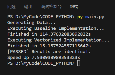
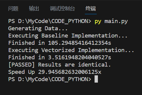
检测实现正确与加速效果