Lab5-简单神经网络训练与加速
实验简介
1
2
3
4
5
6
深度学习(Deep Learning)是机器学习的分支,是一种以人工神经网络为架构,对数据进行表征学习的算法。深度学习 能够取得如此卓越的成就,除了优越的算法、充足的数据,更离不开强劲的算力。近年来,深度学习相关的基础设施逐渐 成熟,从网络设计时的训练、优化,到落地的推理加速,都有非常优秀的解决方案。其中,对于算力的需求最大的部分之 一是网络的训练过程,它也因此成为 HPC 领域经常研究的话题。 本次实验我们将完成 LeNet-5 的训练,并尝试编写自定义算子。
实验环境
在 H248 节点上用 conda activate torch 导入环境
用 sbatch 脚本任务运行程序
1
2
3
4
5
6
7
8
9
#!/bin/bash CUDA_VISIBLE_DEVICES=1 python LeNet-5.py
LeNet-5 训练
1 2 3 4 5 6 7 train_dataset = torchvision.datasets.MNIST(root = '../Lab5/data/' , train = True , transform = transforms.ToTensor(), download = True ) test_dataset = torchvision.datasets.MNIST(root = '../Lab5/data/' , train = False , transform = transforms.ToTensor()) train_loader = torch.utils.data.DataLoader(dataset = train_dataset, batch_size = 64 , shuffle = True ) test_loader = torch.utils.data.DataLoader(dataset = test_dataset, batch_size = 64 , shuffle = False )
1
2
3
4
5
6
7
8
9
10
11
12
13
14
15
16
17
18
19
20
21
22
23
24
25
26
27
28
29
30
31
32
class LeNet5 (nn.Module): def __init__ (self ): super (LeNet5, self).__init__() self.conv1 = nn.Conv2d(in_channels = 1 , out_channels = 6 , kernel_size = 5 , stride = 1 ) self.pool1 = nn.MaxPool2d(kernel_size = 2 , stride = 2 ) self.conv2 = nn.Conv2d(in_channels = 6 , out_channels = 16 , kernel_size = 5 , stride = 1 ) self.pool2 = nn.MaxPool2d(kernel_size = 2 , stride = 2 ) self.fc1 = nn.Linear(in_features = 16 * 4 * 4 , out_features = 120 ) self.fc2 = nn.Linear(in_features = 120 , out_features = 84 ) self.fc3 = nn.Linear(in_features = 84 , out_features = 10 ) def forward (self, x ): x = self.pool1(F.gelu(self.conv1(x))) x = self.pool2(F.gelu(self.conv2(x))) x = x.view(-1 , 16 * 4 * 4 ) x = F.gelu(self.fc1(x)) x = F.gelu(self.fc2(x)) x = self.fc3(x) return x
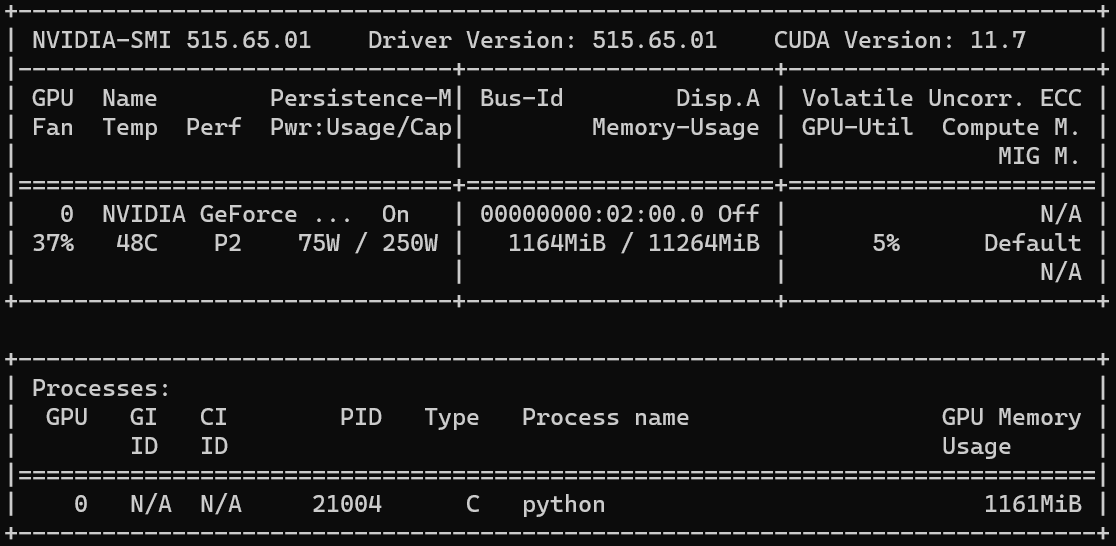
1
2
3
4
device = torch.device("cuda" if torch.cuda.is_available() else "cpu" ) model = LeNet5().to(device) criterion = nn.CrossEntropyLoss().to(device) optimizer = torch.optim.Adam(model.parameters())
1
2
3
4
5
6
7
8
9
10
11
12
13
14
15
for i, (x_train, y_train) in enumerate (train_loader): x_train = x_train.to(device) y_train = y_train.to(device) y_pred = model(x_train) loss = criterion(y_pred, y_train) optimizer.zero_grad() loss.backward() optimizer.step()
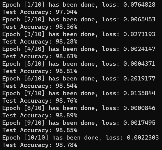
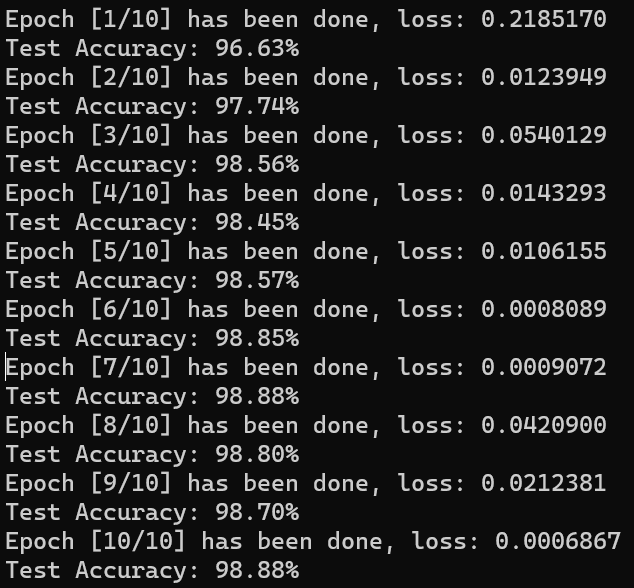
1 2 3 4 5 6 7 8 9 10 11 12 13 14 15 16 17 18 19 20 model.eval () with torch.no_grad(): correct = 0 total = 0 for x_test, y_test in test_loader: x_test = x_test.to(device) y_test = y_test.to(device) y_pred = model(x_test) _, predicted = torch.max (y_pred.data, 1 ) total += y_test.size(0 ) correct += (predicted == y_test).sum ().item() print ('Test Accuracy: {:.2f}%' .format (100 * correct / total))
1 2 3 4 5 6 from torch.utils.tensorboard import SummaryWriterwriter = SummaryWriter('../Lab5/Tensorboard' ) writer.close()
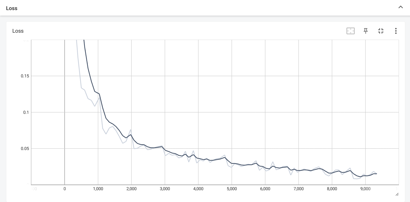
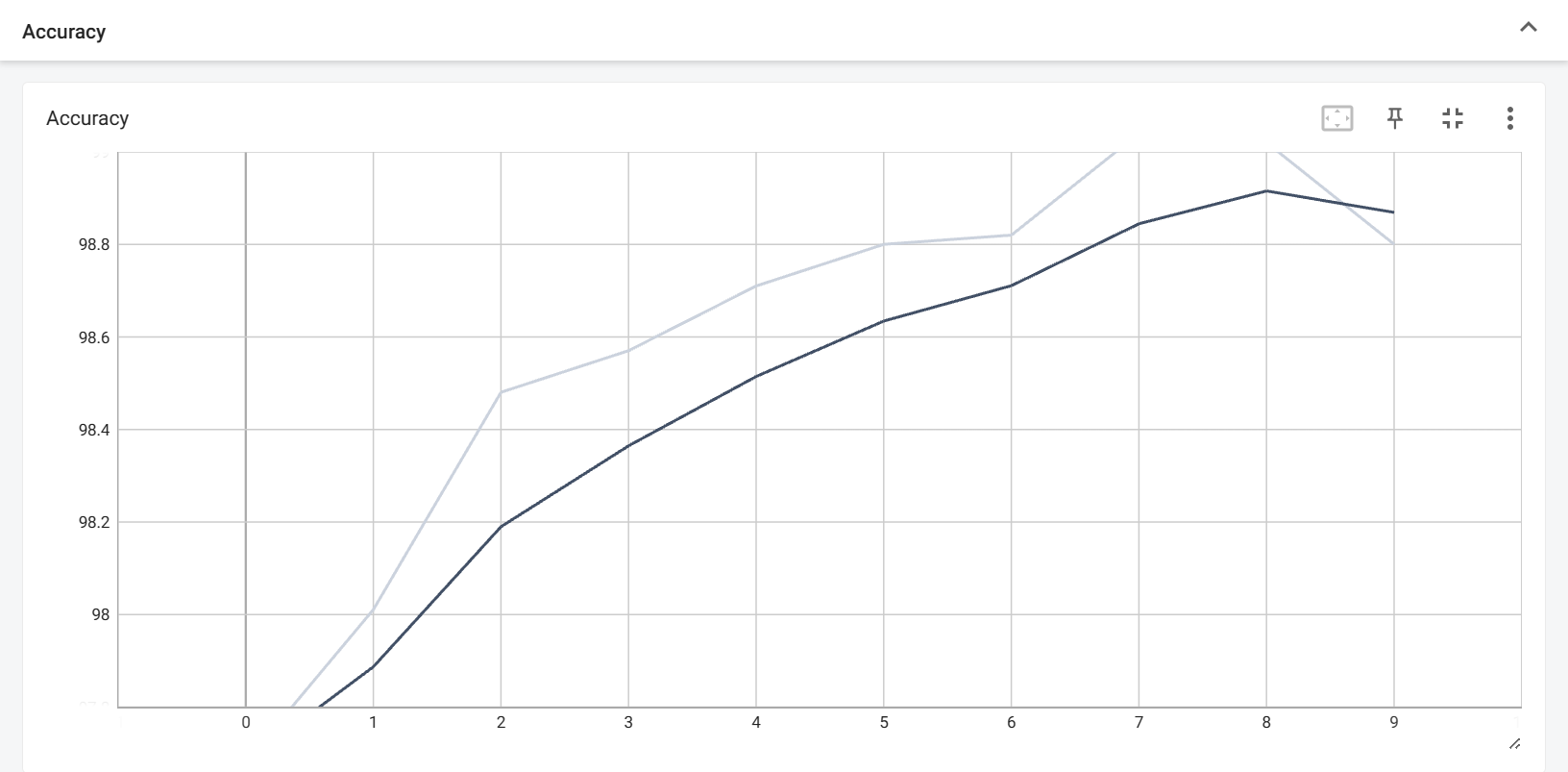
1 2 3 4 writer.add_scalar('Loss' , average_loss / 100 , epoch * len (train_loader) + i) writer.add_scalar('Accuracy' , 100 * correct / total, epoch)
在集群上跑完一次任务后会产生记录文件,使用
tensorboard --logdir=./Lab5/Tensorboard 命令后默认会在
localhost:6006 上打开,本地新建一个终端用
ssh -L 8080:localhost:6006 zsh@clusters.zju.edu.cn -p 80
转发端口,然后在本地浏览器上打开 localhost:8080
就可以看到图像。
编写 GELU 算子
1
2
3
def forward (ctx, input ): ctx.save_for_backward(input ) return 0.5 * input * (1 + torch.tanh(math.sqrt(2 / math.pi) * (input + 0.044715 * torch.pow (input , 3 ))))
\[
\begin{gather*}
\rm{GELU}'(x) = 0.5 * \tanh(0.0356774 * x^3 + 0.797885 * x)\\
+ \rm(0.0535161 * x^3 + 0.398942 * x) * sech^2(0.0356774 * x^3 +
0.797885 * x) + 0.5
\end{gather*}
\]
1
2
3
4
5
6
7
def backward (ctx, grad_output ): input , = ctx.saved_tensors part1 = 0.5 * torch.tanh(0.0356774 * torch.pow (input , 3 ) + 0.797885 * input ) part2 = 0.0535161 * torch.pow (input , 3 ) + 0.398942 * input part3 = 1.0 / (torch.cosh(0.0356774 * torch.pow (input , 3 ) + 0.797885 * input )) grad_input = grad_output * (part1 + part2 * torch.pow (part3, 2 ) + 0.5 ) return grad_input
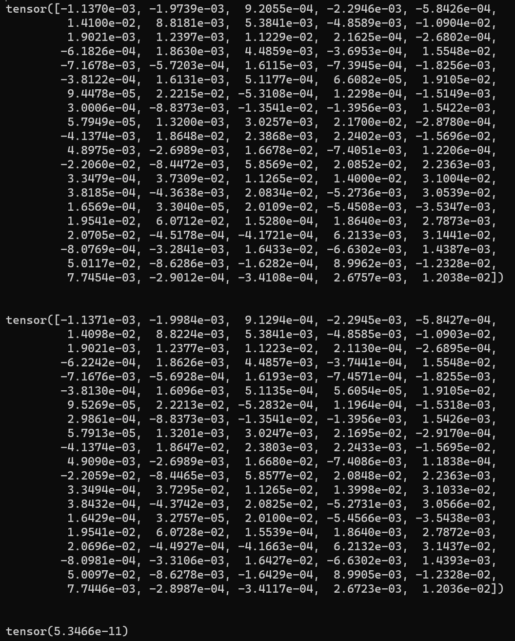
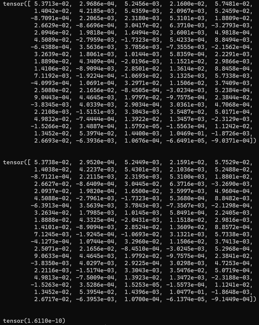
1
2
3
4
5
6
7
8
9
10
11
12
13
14
15
16
17
18
19
A = torch.randn(100 ) B = A.clone() A.requires_grad = True B.requires_grad = True c = torch.randn(100 ) a = F.gelu(A) b = my_gelu(B) loss1 = F.mse_loss(a, c) loss2 = F.mse_loss(b, c) loss1.backward() loss2.backward() gradA = A.grad gradB = B.grad err = F.mse_loss(gradA, gradB) print (gradA)print ('\n' )print (gradB)print ('\n' )print (err)
使用 C++ 算子训练 LeNet-5
文件夹下共有三个文件:setup.py、C_my_gelu.cpp、LeNet-5.py
1
2
3
4
5
6
from setuptools import setup, Extensionfrom torch.utils import cpp_extensionsetup(name = 'C_my_gelu_cpp' , ext_modules = [cpp_extension.CppExtension('C_my_gelu_cpp' , ['C_my_gelu.cpp' ])], cmdclass = {'build_ext' : cpp_extension.BuildExtension})
1 2 3 4 torch::Tensor gelu_forward (const torch::Tensor& input) { return 0.5 * input * (1 + torch::tanh (sqrt (2.0 / pi) * (input + 0.044715 * torch::pow (input, 3 )))); }
1 2 3 4 5 6 7 8 torch::Tensor gelu_backward (const torch::Tensor& input, const torch::Tensor& grad_output) { torch::Tensor part1 = 0.5 * torch::tanh (0.0356774 * torch::pow (input, 3 ) + 0.797885 * input); torch::Tensor part2 = 0.0535161 * torch::pow (input, 3 ) + 0.398942 * input; torch::Tensor part3 = 1.0 / torch::cosh (0.0356774 * torch::pow (input, 3 ) + 0.797885 * input); torch::Tensor grad_input = grad_output * (part1 + part2 * torch::pow (part3, 2 ) + 0.5 ); return grad_input; }
1 2 3 4 5 PYBIND11_MODULE (TORCH_EXTENSION_NAME, m){ m.def ("forward" , &gelu_forward, "gelu forward" ); m.def ("backward" , &gelu_backward, "gelu backward" ); }
1
2
import C_my_gelu_cppfrom torch.autograd import Function
1
2
3
4
5
6
7
8
9
10
11
12
class C_my_gelu (Function ): @staticmethod def forward (ctx, input ): ctx.save_for_backward(input ) return C_my_gelu_cpp.forward(input ) @staticmethod def backward (ctx, grad_output ): input , = ctx.saved_tensors return C_my_gelu_cpp.backward(input , grad_output) my_gelu = C_my_gelu.apply